


A Data Science Case Study With R and mlr
While experimenting with machine learning models, I’ve recently come to enjoy the simplicity and power of OpenML and mlr.
For those new to this, OpenML is a web-based service that provides an entire ecosystem for data scientists. You can easily share and access open data sets from many domains, abstract task and model definitions, and even results shared by other people. One of the nice effects of this service is that you can upload your resulting performance measures and compare your model’s performance to other people’s models.
Secondly, The R-package
mlr provides a
“framework for machine learning experiments”. In short, the package serves as
an interface to many other machine learning packages, with the big advantage of
providing one common syntax. This allows you to quickly try out many different
models from diverse packages without much syntax editing overhead. It is similar
to the caret package, if you know that one. My choice for mlr is based
on a personal bias, though - I have not worked with caret extensively.
I won’t do an extensive tutorial of these packages, since the existing vignette and bootcamp of OpenML and the mlr tutorial and mlr cheatsheet already are excellent resources for that. Instead, I focus on applying these packages in a case study on credit risk.
In this post, I focus on mlr and only use OpenML to download a data set.
A later post, if time allows, describes a workflow using the OpenML functions
and submitting the resulting model to http://www.openml.org
Get a machine learning problem
OpenML defines data objects, tasks, and runs. Data is just a data set, and nothing more. A task is an abstract representation of a problem to be solved by machine learning (it includes the name of the target variable, for example). A run then is the application of one specific machine learning model on a specific task.
Because of that, it usually makes sense to download a task instead of a mere
data set from OpenML. For this analysis, we’ll use pure mlr, though, so
downloading the data set is good enough:
library(OpenML)

d <- getOMLDataSet(data.id = 31)  # this is how you would get a data set

dat <- d$data

dat[1:6, c("job", "purpose", "duration", "credit_amount", "class")]
## job purpose duration credit_amount class
## 0 skilled radio/tv 6 1169 good
## 1 skilled radio/tv 48 5951 bad
## 2 unskilled resident education 12 2096 good
## 3 skilled furniture/equipment 42 7882 good
## 4 skilled new car 24 4870 bad
## 5 unskilled resident education 36 9055 good
This data set contains observations of credit applications. The variables
include a person’s employment, the credit amount, the duration of the credit,
and many others. The target variable is called class and represents whether
the person is of “good” or “bad” credit status, where “bad” hints at a possible
default of the loan. Banks then want to predict this status and base their
decision on whether or not to grant the loan on the status prediction.
Exploratory data analysis
Of course, in a real setting you would now take some time to get used to the data. This would include summaries and plots, both univariate and multivariate.
As an example, here I’ll plot the density estimation for the credit amount, separately for the good and bad classes:
library(ggplot2)
ggplot(dat, aes(x=credit_amount, group=class, colour=class)) + geom_density() +
  ggtitle("Density of requested credit amount, grouped by class (good/bad)")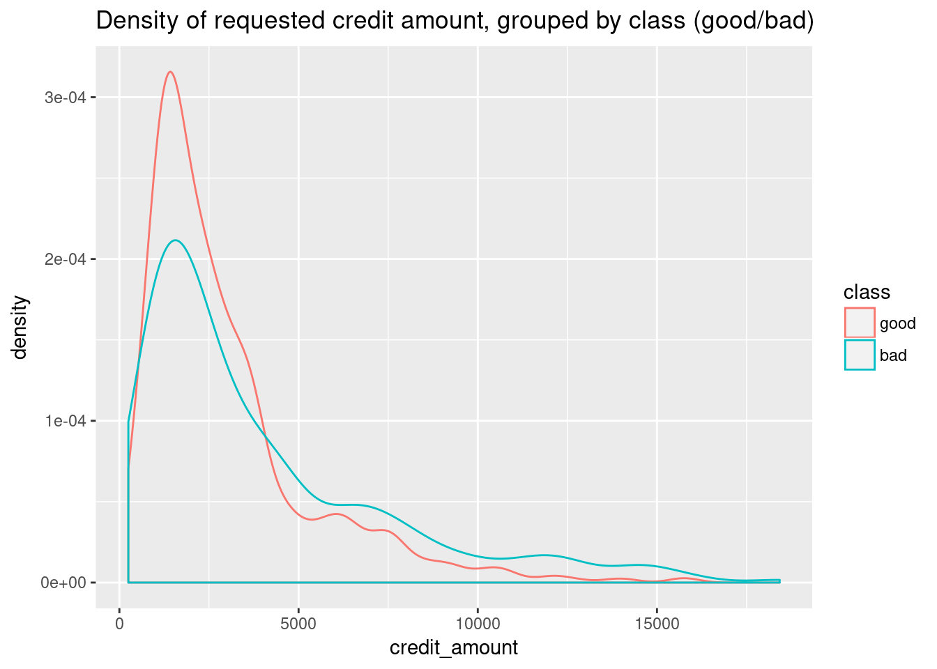
Here, you already get a feeling that higher credit amounts tend to default more often, and thus might be classified as “bad” more easily.
Running machine learning models
First, we will run a binomial regression to predict a credit applicant’s risk class.
There are two ways to proceed here. Either we run within the mlr framework,
or we use the OpenML functions. I’ll stick with mlr to keep the set of
introduced functions as small as possible - there might be a different post
using OpenML at a later point, though.
library(mlr)

task <- makeClassifTask(data = dat, target = "class")
glm.learner <- makeLearner("classif.binomial")

task
## Supervised task: dat
## Type: classif
## Target: class
## Observations: 1000
## Features:
## numerics factors ordered functionals
## 7 13 0 0
## Missings: FALSE
## Has weights: FALSE
## Has blocking: FALSE
## Classes: 2
## good bad
## 700 300
## Positive class: good
The task contains the data set, the problem type (classification), the target
variable, among others. Important is also the information which class is
considered the “positive” class (here: good credit rating), since this affects
how we interpret measures like the true positive rate later.
Now we are ready to train the binomial learner. We’ll also use it to predict the outcome for the held back test set, and check a few common performance measures to see how the model did:
n <- nrow(dat)
set.seed(20171119)
train.id <- sample(n, size = 2/3*n)
test.id <- setdiff(1:n, train.id)
glm.model <- train(glm.learner, task, subset = train.id)

pred <- predict(glm.model, task, subset = test.id)

table(pred$data[,2:3])
## response
## truth good bad
## good 195 36
## bad 48 55
performance(pred, measures=list(acc, tpr, fpr, fnr))## acc tpr fpr fnr
## 0.7485030 0.8441558 0.4660194 0.1558442
Oh that’s not good! The false positive rate is 0.47! Here, positive means that a subject has a good credit class. This means that the FPR is interpreted as the ratio of people with bad credit that falsely get classified as “good credit”. This is fatal, since we would give out loans to almost half of the people who are actually of a “bad” credit status.
Since we only predicted a class here, we should check if a different threshold cutoff (say, 0.8 instead of 0.5) can be of help. This would mean that our model would become more conservative, in the sense that it would put more people in the “bad” class.
Predicting probability instead of class
mlr has convenient functions for plotting how a model’s performance responds
to differing thresholds. We create a new task that predicts the probability
instead of the class directly, and plot its performance versus the threshold
probability for class="bad":
glm.prob.learner <- makeLearner("classif.binomial", predict.type = "prob")
glm.prob.model <- train(glm.prob.learner, task, subset = train.id)
pred <- predict(glm.prob.model, task, subset = test.id)
d <- generateThreshVsPerfData(pred, measures = list(fpr, fnr, mmce))
plotThreshVsPerf(d)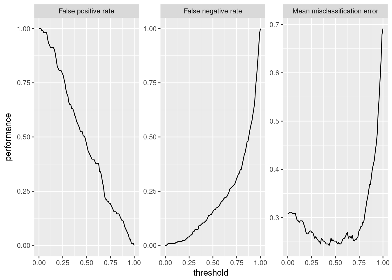
The misclassification error seems “okay” for a threshold from 0.10 to around 0.80. For us, a false positive happens when someone that is actually a bad credit gets classified as “good credit”. This ratio is more important to us, since here, we would give someone a loan that will probably default on it.
A false negative, on the other hand, would be someone of “good” credit status that we wrongly classify as “bad credit”. This mistake is also not optimal, but, financially, not nearly as bad as a false positive.
Thus, we aim to keep the FPR as low as possible while still aiming to keep a well performing model. Visually, a threshold of around 0.70 seems reasonable, since the total misclassification is still under 30%, while the FPR is now under 25%.
However, we still give out loans to one out of four people with a “bad” rating. Is there any chance for further improvement? Maybe a different algorithm, such as a random forest, provides a better performance?
Tuning a random forest
Let’s compare other models’ performances. The listLearners() function shows
you which models are already available in mlr:
listLearners()[1:6, 1:4]## class name short.name package
## 1 classif.ada ada Boosting ada ada,rpart
## 2 classif.bartMachine Bayesian Additive Regression Trees bartmachine bartMachine
## 3 classif.binomial Binomial Regression binomial stats
## 4 classif.blackboost Gradient Boosting With Regression Trees blackboost mboost,party
## 5 classif.boosting Adabag Boosting adabag adabag,rpart
## 6 classif.bst Gradient Boosting bst bst,rpart
A random forest is implemented in the classif.ranger class. This is from the
ranger package, a faster implementation of random forests.
Larger tuning tasks can take up a larger amount of CPU time. Luckily, mlr
works well together with the parallelMap package (it comes from the same
authors). Basic parallelization of model tuning works out-of-the-box with little
additional code.
In the following bit of code, we tune a random forest by performing a random
search for the optimal value for num.trees, i.e. the number of trees to grow
(from 100 to 1000), and mtry, the optimal number of variables to consider at
each split.
library("parallelMap")
parallelStartSocket(3)

ranger.learner <- makeLearner("classif.ranger", predict.type = "prob")

ps <- makeParamSet(
  makeIntegerParam("num.trees", lower=100, upper=1000),
  makeIntegerParam("mtry", lower=2, upper=15)
)
ctrl <- makeTuneControlRandom(maxit = 100)
rdesc <- makeResampleDesc("CV", iters = 3)
res <- tuneParams("classif.ranger", task = task, resampling = rdesc,
                  par.set = ps, control = ctrl, measure = acc)
parallelStop()
res$x
## $num.trees
## [1] 764
##
## $mtry
## [1] 13
So, according to a random search, it seems that a random forest with 764
trees and an mtry of 13 is the best option to proceed with (if
you care mostly about accuracy).
You can even plot the effects of hyperparameters, e.g. in a heat map where missing data (and there is a lot of it) is interpolated with another random forest:
hped <- generateHyperParsEffectData(res)
plotHyperParsEffect(hped, x="num.trees", y="mtry", z="acc.test.mean",
                    plot.type="heatmap", interpolate = "regr.ranger")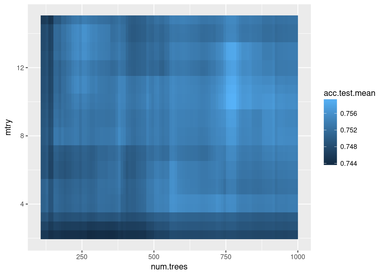
This plot would be more helpful if I had tuned on a denser grid, i.e. more than 100 random points - the interpolation is very noisy here.
Benchmarking different models
Next, we’ll use the results from our tuning experiment and compare the binomial
model against the tuned random forest. In mlr, the benchmark() function
takes care of this:
tuned.ranger.learner <- makeLearner("classif.ranger", predict.type = "prob",
                                    num.trees = best.n, mtry = best.mtry)

learnersList <- list(
  glm.prob.learner,
  tuned.ranger.learner
)

rdesc <- makeResampleDesc("CV", iters = 10, predict = "test")
bmr <- benchmark(learnersList, task, rdesc,
                 measures = list(fpr, fnr, acc, mmce, timetrain))

getBMRAggrPerformances(bmr, as.df=TRUE)
## task.id learner.id fpr.test.mean fnr.test.mean acc.test.mean mmce.test.mean timetrain.test.mean
## 1 dat classif.binomial 0.4889297 0.1318035 0.759 0.241 0.0386
## 2 dat classif.ranger 0.5299881 0.1078258 0.761 0.239 0.7362
The misclassification error (mmce, which is 1 - accuracy) is just slightly
lower for the random forest. There is a bigger difference, however, in that the
random forest’s false negative rate is lower, but the false positive rate
is higher.
Because for credit risk, a false positive is way worse than a false negative, we should focus on keeping the FPR as low as possible. Currently, the logistic regression model is doing a better job at this.
Apply different probability thresholds
Earlier we saw that for the binomial classification, we should set the probability threshold up to something in the vicinity of 0.70, in order to make our model more conservative. We can do so by another convenient one-liner and benchmark the models again:
tuned.ranger.learner <- setPredictThreshold(tuned.ranger.learner, 0.70)
tuned.glm.learner <- setPredictThreshold(glm.prob.learner, 0.70)

learnersList <- list(
  tuned.glm.learner,
  tuned.ranger.learner
  )
bmr <- benchmark(learnersList, task, rdesc,
                 measures = list(fpr, fnr, acc, mmce, timetrain))

getBMRAggrPerformances(bmr, as.df=TRUE)
## task.id learner.id fpr.test.mean fnr.test.mean acc.test.mean mmce.test.mean timetrain.test.mean
## 1 dat classif.binomial 0.3179700 0.2774737 0.714 0.286 0.0276
## 2 dat classif.ranger 0.2375624 0.3452514 0.689 0.311 0.7745
Oh look! If we set our algorithms to be more conservative (i.e., to only give out a “good” prediction if the probability for good is greater than 0.70), now the random forest outperforms the GLM with an FPR of 0.24 versus 0.32, at the cost of a slightly higher misclassification error (0.31 vs. 0.29).
We have arrived at a tuned, conservative random forest with a false positive
rate of just 0.24.
There is probably still much room for improvement (almost a third of all people
still get misclassified), but that is outside of the scope of this short
introduction. Nonetheless, I hope I’ve demonstrated the simplicity and strength
of the mlr package.
Other things not touched upon in this article
This article is a first experiment with mlr and the package has much more
power than I’ve outlined here. Here are some other interesting features:
Feature selection is the task of choosing a small and informative subset of
input variables (features) from the data set to keep the model interpretable
and speed up the learning time. In mlr, this is called filtering and
described in a [tutorial article]
(https://mlr-org.github.io/mlr-tutorial/devel/html/feature_selection/index.html).
If your data has missing values and you want to impute them, mlr offers convenient one-liners to impute an entire data set, either by simple functions such as the mode or the mean, or with models such as classification trees. The corresponding tutorial article describes how to do this.
Also, a more elaborate procedure for dealing with the fact that a false positive is more important to avoid than a false negative is called cost-sensitive classification. For example, the following cost matrix for the credit data set says that it’s 5 times worse to classify a person with bad risk as good than vice-versa:
##      Good Bad
## Good    0   1
## Bad     5   0
The mlr tutorial (again) has an excellent article on this online.